The Four Essential System Properties for Signal Processing

Understanding different properties of a given system is essential to truly understand the system under consideration and derive the output of such a system for any input of our choice. In this blog, we will take a detailed look at four fundamental properties of a system, namely Shift in-variance, Linearity, Causality, and BIBO Stability.

Time varying signal

Shift Invariance

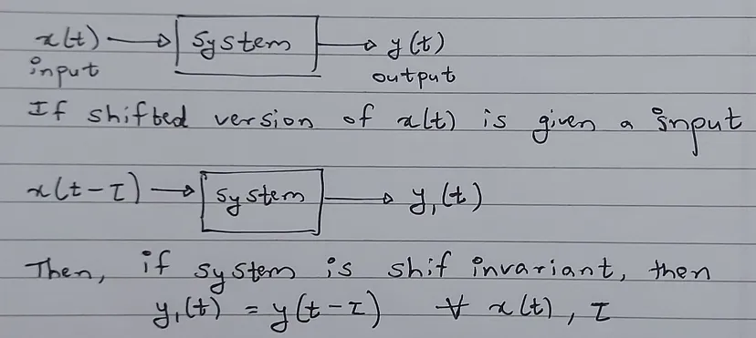
If the input given to a system is shifted and if the output of the system also gets shifted by the same amount, then the system is said to be shift invariant. Let us illustrate this through an example.

Theoretical Definition of Shift Invariance

y(t) = x(2t)

If we shift x(t) by a units, then we get x(t - a). If this is given as input
to the system, the output will be y1 = x(2(t - a)). But if we shift y(t)
by a units then we get y2 = x(2t - a). We can clearly see that y1 is not equal
to y2 for all x(t) and thus the system is not Shift Invariant.

Linearity

If a system obeys the following 2 properties then it is said to be a linear system.

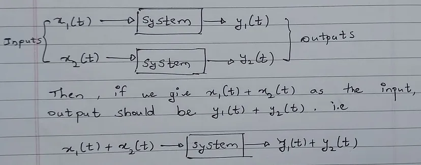
Additivity

Mathematical definition of Additivity

The above condition must be true for all x(t). Let us take an example.

1. Let, y(t) = 3x(t)
So, y1(t) = 3x1(t) and y2(t) = 3x2(t).
Now, if we give x1(t) + x2(t) as the input, then the output is-
y(t) = 3{x1(t) + x2(t)} = 3x1(t) + 3x2(t) = y1(t) + y2(t). Thus the system is
Additive

2. Let y(t) = x(t) + 5
So, y1(t) = x1(t) + 5 and y2(t) = x2(t) + 5.
Now, if we give x1(t) + x2(t) as the input then output is-
y(t) = {x1(t) + x2(t)} + 5.
But, y1(t) + y2(t) = {x1(t) + 5} + {x2(t) + 5} = {x1(t) + x2(t)} + 10.
Thus, we can see that y(t) is not equal to y1(t) + y2(t) and thus the system
is not Additive.

Homogeneity

Mathematical Definition of a homogeneous system

Let us take some examples to make the definition clear and easy to understand.

1. y(t) = x(t)
If we give input as x1(t) = 3x(t), then output will be-
y1(t) = x1(t) = 3x(t) = 3y(t). Thus when the input is multiplied by 3, output
is also multiplied by 3 and the system is indeed homogeneous.

2. y(t) = 2x(t) + 3
If we give input as x1(t) = 7x(t), then the output will be-
y1(t) = 2x1(t) + 3 = 14x(t) + 3. But, 
7y(t) = 14x(t) + 21.
We can clearly see that y1(t) is not equal to 7y(t) and thus this system is
not homogeneous.

If a system is both Additive and Homogeneous then it is said to be a Linear System.

LTI Systems

LTI means a Linear and Shift Invariant system. Thus if a system is LTI then, it must be both Linear and Shift Invariant. LTI system, show some amazing properties and we will discuss them in great detail in future blogs.

Causality (effect should not precede the cause)

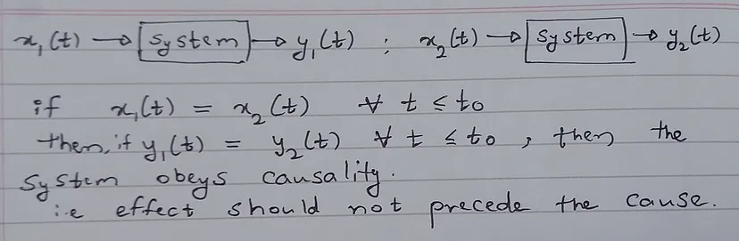
Causality means obeying cause-effect relationship. Here we assume temporal nature of the independent variable. {In most cases, time is the independent variable.}

Mathematical Definition of Causality

The above definition might seem obvious but let us take some examples to make sure we appreciate it’s importance.

1. y(t) = 13x(t - 1)
Then, we have y1(t) = 13x1(t - 1) and y2(t) = 13x2(t - 1). Now let us say,
we give the same input a(t) to both the systems till t = 10s. Then, as both
y1(t) and y2(t) depend on inputs at 1 time step before, we can see that 
y1(t) = y2(t) till t = 11s. We don't know their behaviour after t = 11s but 
we can guarantee that they will be the same till atleast t = 10s. Thus the
given system is causal.

2. y(t) = x(t + 1)
Then, we have y1(t) = x1(t + 1) and y2(t) = x2(t + 1). Now let us say,
we give the same input a(t) to both the systems till t = 10s. But we can see
that we cannot say y1(t) = y2(t) till t= 10s because at t = 10s both
y1(t) and y2(t) depend on the inputs at t = 11s and we don't know whether
they x1(t) = x2(t) at t = 11s. Thus this system is not causal.

BIBO Stability

BIBO stability {Bounded Input Bounded Output Stability} simply means that the system will always produce bounded (finite) output when presented by a bounded (finite) input. This does not guarantee the behaviour of the system {whether it will provide a bounded or an unbounded output} when given an unbounded(infinite) input.

Definition of boundedness for a time varying signal

There are many different notions of stability for a time varying signal but BIBO stability is a widely used and discussed measure of stability in the literature of Signal Processing. Let us take some examples.

1. y(t) = sin(7x(t) + 1000)
Here let, x(t) be bounded by a constant M. Then, the argument of sin will vary
in range -> [1000 - 7M, 1000 + 7M] and no matter what is the argument, sin
will always be in range -> [-1, 1]. Thus the output is Bounded if the input 
is bounded and thus the system is BIBO stable. {Here infact the output is 
always bouded irrespective of the boundedness of the input}

2. y(t) = tan(x(t))
Let us assume that x(t) is bounded by a constant M = pi.
Then x(t) will vary in range -> [-pi, pi].
We know that tan({pi/2}) is infinity and thus when x(t) = pi/2, the output
becomes unbounded even though the input is bounded. Thus above system is 
not BIBO Stable.

Checking if the system under consideration is stable or not, is very important for the practical realisation of our system, as we cannot design systems which have an unbounded output for a given bounded input of our interest.

Congratulations, you made it to the end of this Blog! I hope you enjoyed reading it and got better insights into the most fundamental properties of a time varying system. Here, we only discussed the analysis of the system in time domain. We can analyse systems in frequency domain and also by making use of the impulse response (A very powerful tool in Signal Processing) of a system but these are the topics of separate blogs and will be discussed in the future. Till then, Goodbye and keep enjoying the world of Signal Processing.